Shiny从入门到入定——8-用户反馈

蛋白质组的全局 pIs

细胞全局蛋白质组 pI 图的变化取决于氨基酸的总电荷，并对蛋白质的结构和特性具有重要意义。

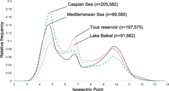
普遍认为原核基因组具有两个最大的双峰形状，一个在酸性pH值下主要对应于溶解的蛋白质（细胞质蛋白或分泌蛋白），另一种在膜蛋白的碱性pH值下，具有细胞内碱性（带正电荷）结构域以促进质子动力的产生。在这两个峰之间，有一个最小的中性值，对应于细胞内的pH值（如下图）。

蛋白质氨基酸组成和 pI 水平的显着变化提供了一种工具来预测培养物或宏基因组组装基因组(MAG)的首选栖息地。

Pedro J. et al., 2019, Microbiome

安装EMBOSS

• 下载

wget  ftp://emboss.open-bio.org/pub/EMBOSS/emboss-latest.tar.gz

• 安装

# 解压
tar zxvf emboss-latest.tar.gz

# 防止报错 (error while loading shared libraries: libnucleus.so.6)
sudo /sbin/ldconfig

# 配置、编译与安装
cd emboss-latest
./configure
make
sudo make install

输入文件

输入文件为含有一条或多条氨基酸序列的FASTA格式文件。

计算氨基酸序列的各特征数据Calculate statistics of protein properties

逐个文件计算

pepstats -sequence F01_bin.1.faa -outfile F01_bin.1.out

:::primary 参数解析

• Standard (Mandatory) qualifiers:

  • [-sequence] seqall Protein sequence(s) filename and optional
    format, or reference (input USA)
  • [-outfile] outfile [*.pepstats] Pepstats program output file

• Advanced (Unprompted) qualifiers:

  • -aadata datafile [Eamino.dat] Amino acid properties
  • -mwdata datafile [Emolwt.dat] Molecular weight data for amino
    acids
  • -pkdata datafile [Epk.dat] Values of pKa for amino acids
  • -[no]termini boolean [Y] Include charge at N and C terminus
  • -mono boolean [N] Use monoisotopic weights

:::

批量计算与pI提取并输出为相对丰度

#!/usr/bin/perl
use strict;
use warnings;
# name: print_pI.pl
# Author: Liu Hualin
# Date: 2022.01.03

my @genome = glob("*.faa");
foreach  (@genome) {
	$_=~/(\S+).faa/;
	my $out = $1 . ".pepstats";
	my $pi = $1 . ".pI";
	system("pepstats -sequence $_ -outfile $out");

	my %hash;
	my $seqnum = 0;
	open IN, "$out" || die;
	while (<IN>) {
		chomp;
		if (/^(Isoelectric Point = )(\S+)/) {
			my $pi = sprintf "%.1f", $2;
			$hash{$pi}++;
			$seqnum++;
		}
	}
	close IN;

	#my @records = values %hash;
	#my $seqnum = @records;
	#print $seqnum . "\n";
	open OUT, ">$pi" || die;
	print OUT "Isoelectric point\tRelative frequency\n";
	foreach  (keys %hash) {
		my $frequency = sprintf "%.2f", $hash{$_}/$seqnum;#@records;
		print OUT "$_\t$frequency\n";
	}
	close OUT;
}

选择性忽略 （这是我自己用的）

#!/usr/bin/perl
use strict;
use warnings;
# name: co_sample_pI.pl
# Author: Liu Hualin
# Date: 2022.01.03

open OUT, ">F06.pi" || die;
print OUT "MAGs\tIsoelectric point\tRelative frequency\n";
my @pI = glob("F06*.pI");
foreach  (@pI) {
	$_=~/(\S+).pI/;
	my $mag = $1;
	open IN, "$_" || die;
	<IN>;
	while (<IN>) {
		chomp;
		print OUT "$mag\t$_\n";
	}
	close IN;
}
close OUT;

可视化

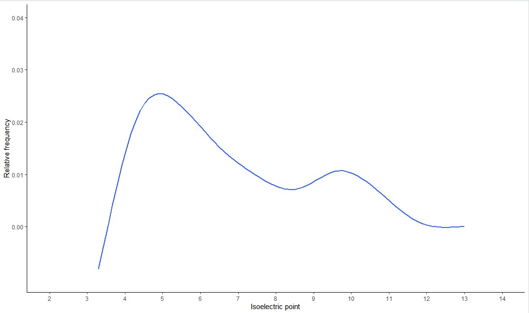
绘制蛋白质组的全局 pIs图

# Step 1 读入数据
setwd("E:/Researches/Xiaqian/NGS/CleanData/宏基因组数据/Result/Results/Annotations/AAs")

F1 <-read.table("F01_bin.1.pI", sep = "\t", header = T)

# Step 2 绘图，以下5选1
## 单组加点，运行完后跳到Step 3
p1 <- ggplot(F1, aes(Isoelectric.point, Relative.frequency))+geom_point(size=2,shape=21)+geom_smooth(method= "gam")+theme_classic()

## 单组无点，运行完后跳到Step 3
p1 <- ggplot(F1, aes(Isoelectric.point, Relative.frequency))+geom_smooth(method= "gam")+theme_classic()


## 多组加点
p1 <- ggplot(F1, aes(Isoelectric.point, Relative.frequency, color=MAGs))+geom_point(size=3,shape=21)+geom_smooth(method= "gam")+theme_classic()


## 多组无点显示置信区间
p1 <- ggplot(F1, aes(Isoelectric.point, Relative.frequency, color=MAGs))+geom_smooth(method= "gam")+theme_classic()

## 多组无点去除置信区间
p1 <- ggplot(F1, aes(Isoelectric.point, Relative.frequency, color=MAGs))+geom_smooth(method= "gam",se = FALSE)+theme_classic()


# Step 3 美化，看下图
p1 + scale_x_continuous(limits=c(2, 14), breaks = seq(2, 14, 1))+ scale_y_continuous(limits=c(-0.01, max(F1$Relative.frequency)), breaks = seq(0,max(F1$Relative.frequency), 0.01))+ labs(x= "Isoelectric point",y = "Relative frequency")

## ==============以下代码为自用========================
## F04自定义颜色
p1 + scale_x_continuous(limits=c(2, 14), breaks = seq(2, 14, 1))+ scale_y_continuous(limits=c(-0.01, max(F1$Relative.frequency)), breaks = seq(0,max(F1$Relative.frequency), 0.01))+ labs(x= "Isoelectric point",y = "Relative frequency")+ scale_color_manual(name="MAGs", values=c("#1f77b4","#ff7f0e","#2ca02c", "#d62728", "#9467bd", "#8c564b", "#e377c2", "#bcbd22"))

## F05自定义颜色
p1 + scale_x_continuous(limits=c(2, 14), breaks = seq(2, 14, 1))+ scale_y_continuous(limits=c(-0.01, max(F1$Relative.frequency)), breaks = seq(0,max(F1$Relative.frequency), 0.01))+ labs(x= "Isoelectric point",y = "Relative frequency")+ scale_color_manual(name="MAGs", values=c("#1f77b4","#ff7f0e","#2ca02c", "#d62728", "#9467bd", "#8c564b", "#e377c2", "#bcbd22", "#17becf"))

## F06自定义颜色
p1 + scale_x_continuous(limits=c(2, 14), breaks = seq(2, 14, 1))+ scale_y_continuous(limits=c(-0.01, max(F1$Relative.frequency)), breaks = seq(0,max(F1$Relative.frequency), 0.01))+ labs(x= "Isoelectric point",y = "Relative frequency")+ scale_color_manual(name="MAGs", values=c("#1f77b4","#ff7f0e","#2ca02c", "#d62728", "#9467bd", "#8c564b", "#e377c2", "#bcbd22", "#17becf", "#f7b6d2", "#5254a3", "#000000"))

参考

• Pedro J. et al., 2019, Microbiome

• EMBOSS

代码获取

关注公众号“生信之巅”，聊天窗口回复“85d7”获取下载链接。

敬告：使用文中脚本请引用本文网址，请尊重本人的劳动成果，谢谢！Notice: When you use the scripts in this article, please cite the link of this webpage. Thank you!