简介 本文构建预测员工是否会离职的模型,并使用模型对员工进行预测。通过本文可以学习到:
查看数据集的统计信息
特征工程
数据集的划分
数据集的预处理
数据集的可视化
模型训练
模型调参
模型评估
模型预测
查看数据集信息 1 2 3 4 5 6 7 8 9 import numpy as npimport pandas as pdurl = 'https://cdn.jsdelivr.net/gh/liaochenlanruo/cdn@master/data/ML/HumanResourcesAnalytics/HR_comma_sep.csv' df = pd.read_csv(url) print (df.info()) df.head()
<class 'pandas.core.frame.DataFrame'>
RangeIndex: 14999 entries, 0 to 14998
Data columns (total 10 columns):
# Column Non-Null Count Dtype
--- ------ -------------- -----
0 satisfaction_level 14999 non-null float64
1 last_evaluation 14999 non-null float64
2 number_project 14999 non-null int64
3 average_montly_hours 14999 non-null int64
4 time_spend_company 14999 non-null int64
5 Work_accident 14999 non-null int64
6 left 14999 non-null int64
7 promotion_last_5years 14999 non-null int64
8 sales 14999 non-null object
9 salary 14999 non-null object
dtypes: float64(2), int64(6), object(2)
memory usage: 1.1+ MB
None
satisfaction_level
last_evaluation
number_project
average_montly_hours
time_spend_company
Work_accident
left
promotion_last_5years
sales
salary
0
0.38
0.53
2
157
3
0
1
0
sales
low
1
0.80
0.86
5
262
6
0
1
0
sales
medium
2
0.11
0.88
7
272
4
0
1
0
sales
medium
3
0.72
0.87
5
223
5
0
1
0
sales
low
4
0.37
0.52
2
159
3
0
1
0
sales
low
header 信息
satisfaction_level 员工满意度
last_evaluation 员工考核评分
number_project 员工参与的项目数
average_montly_hours 每个月均工作时长
time_spend_company 员工工作年限
Work_accident 是否发生过事故
left 员工是否离职
promotion_last_5years 过去5年中是否有升职
sales 员工岗位
salary 员工薪资水平
1 2 3 4 df.rename(columns={'average_montly_hours' :'average_monthly_hours' , 'sales' :'department' }, inplace=True ) df.head()
satisfaction_level
last_evaluation
number_project
average_monthly_hours
time_spend_company
Work_accident
left
promotion_last_5years
department
salary
0
0.38
0.53
2
157
3
0
1
0
sales
low
1
0.80
0.86
5
262
6
0
1
0
sales
medium
2
0.11
0.88
7
272
4
0
1
0
sales
medium
3
0.72
0.87
5
223
5
0
1
0
sales
low
4
0.37
0.52
2
159
3
0
1
0
sales
low
satisfaction_level
last_evaluation
number_project
average_monthly_hours
time_spend_company
Work_accident
left
promotion_last_5years
count
14999.000000
14999.000000
14999.000000
14999.000000
14999.000000
14999.000000
14999.000000
14999.000000
mean
0.612834
0.716102
3.803054
201.050337
3.498233
0.144610
0.238083
0.021268
std
0.248631
0.171169
1.232592
49.943099
1.460136
0.351719
0.425924
0.144281
min
0.090000
0.360000
2.000000
96.000000
2.000000
0.000000
0.000000
0.000000
25%
0.440000
0.560000
3.000000
156.000000
3.000000
0.000000
0.000000
0.000000
50%
0.640000
0.720000
4.000000
200.000000
3.000000
0.000000
0.000000
0.000000
75%
0.820000
0.870000
5.000000
245.000000
4.000000
0.000000
0.000000
0.000000
max
1.000000
1.000000
7.000000
310.000000
10.000000
1.000000
1.000000
1.000000
1 2 3 4 5 print ('Departments:' )print (df['department' ].value_counts())print ('\nSalary:' )print (df['salary' ].value_counts())
Departments:
department
sales 4140
technical 2720
support 2229
IT 1227
product_mng 902
marketing 858
RandD 787
accounting 767
hr 739
management 630
Name: count, dtype: int64
Salary:
salary
low 7316
medium 6446
high 1237
Name: count, dtype: int64
1 2 3 4 5 6 7 8 9 10 11 12 13 14 ''' satisfaction_level | Satisfaction level of employee based on survey | Continuous | [0.09, 1] last_evaluation | Score based on employee's last evaluation | Continuous | [0.36, 1] number_project | Number of projects | Continuous | [2, 7] average_monthly_hours | Average monthly hours | Continuous | [96, 310] time_spend_company | Years at company | Continuous | [2, 10] Work_accident | Whether employee had a work accident | Categorical | {0, 1} left | Whether employee had left (Outcome Variable) | Categorical | {0, 1} promotion_last_5years | Whether employee had a promotion in the last 5 years | Categorical | {0, 1} department | Department employee worked in | Categorical | 10 departments salary | Level of employee's salary | Categorical | {low, medium, high} '''
1 "\nsatisfaction_level | Satisfaction level of employee based on survey | Continuous | [0.09, 1]\nlast_evaluation | Score based on employee's last evaluation | Continuous | [0.36, 1]\nnumber_project | Number of projects | Continuous | [2, 7]\naverage_monthly_hours | Average monthly hours | Continuous | [96, 310]\ntime_spend_company | Years at company | Continuous | [2, 10]\nWork_accident | Whether employee had a work accident | Categorical | {0, 1}\nleft | Whether employee had left (Outcome Variable) | Categorical | {0, 1}\npromotion_last_5years | Whether employee had a promotion in the last 5 years | Categorical | {0, 1}\ndepartment | Department employee worked in | Categorical | 10 departments\nsalary | Level of employee's salary | Categorical | {low, medium, high}\n"
特征工程
查找相关性大的特征,只保留其中的一个。
也可查看与标签(left)相关性较大的特征,如此数据集中的satisfaction_level。
1 2 3 4 numeric_df = df.select_dtypes(include=[np.number]) numeric_df.corr()
satisfaction_level
last_evaluation
number_project
average_monthly_hours
time_spend_company
Work_accident
left
promotion_last_5years
satisfaction_level
1.000000
0.105021
-0.142970
-0.020048
-0.100866
0.058697
-0.388375
0.025605
last_evaluation
0.105021
1.000000
0.349333
0.339742
0.131591
-0.007104
0.006567
-0.008684
number_project
-0.142970
0.349333
1.000000
0.417211
0.196786
-0.004741
0.023787
-0.006064
average_monthly_hours
-0.020048
0.339742
0.417211
1.000000
0.127755
-0.010143
0.071287
-0.003544
time_spend_company
-0.100866
0.131591
0.196786
0.127755
1.000000
0.002120
0.144822
0.067433
Work_accident
0.058697
-0.007104
-0.004741
-0.010143
0.002120
1.000000
-0.154622
0.039245
left
-0.388375
0.006567
0.023787
0.071287
0.144822
-0.154622
1.000000
-0.061788
promotion_last_5years
0.025605
-0.008684
-0.006064
-0.003544
0.067433
0.039245
-0.061788
1.000000
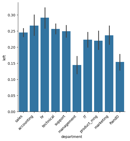
1 2 3 4 5 6 7 import matplotlib.pyplot as pltimport seaborn as sns%matplotlib inline plot = sns.catplot(x='department' , y='left' , kind='bar' , data=df) plot.set_xticklabels(rotation=45 , horizontalalignment='right' );
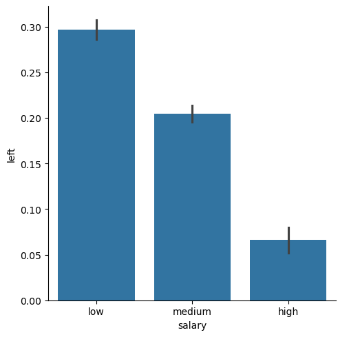
1 2 plot = sns.catplot(x='salary' , y='left' , kind='bar' , data=df);
1 2 df[df['department' ]=='management' ]['salary' ].value_counts().plot(kind='pie' , title='Management salary level distribution' );
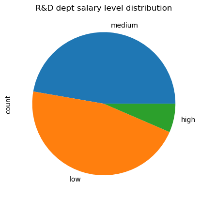
1 2 df[df['department' ]=='RandD' ]['salary' ].value_counts().plot(kind='pie' , title='R&D dept salary level distribution' );
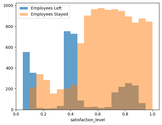
1 2 3 4 5 6 7 8 9 10 11 bins = np.linspace(0.0001 , 1.0001 , 21 ) plt.hist(df[df['left' ]==1 ]['satisfaction_level' ], bins=bins, alpha=0.7 , label='Employees Left' ) plt.hist(df[df['left' ]==0 ]['satisfaction_level' ], bins=bins, alpha=0.5 , label='Employees Stayed' ) plt.xlabel('satisfaction_level' ) plt.xlim((0 ,1.05 )) plt.legend(loc='best' );
发现已离职员工对公司的满意度比较低(0~0.5),当然也存在满意度较高(0.8附近)的员工离职的情况。
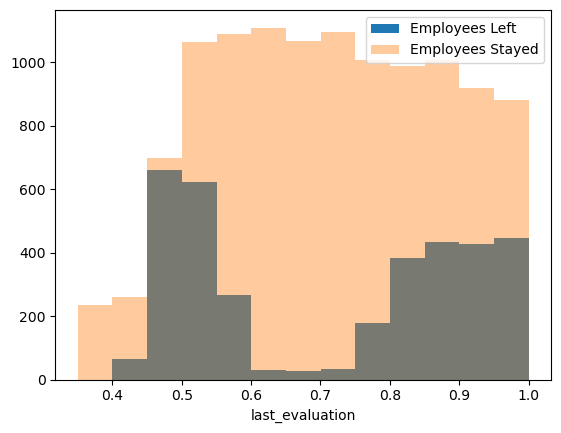
1 2 3 4 5 6 bins = np.linspace(0.3501 , 1.0001 , 14 ) plt.hist(df[df['left' ]==1 ]['last_evaluation' ], bins=bins, alpha=1 , label='Employees Left' ) plt.hist(df[df['left' ]==0 ]['last_evaluation' ], bins=bins, alpha=0.4 , label='Employees Stayed' ) plt.xlabel('last_evaluation' ) plt.legend(loc='best' );
公司评分高(0.8~1.0)的员工离职了很多,原因可能是这部分员工能力强,跳槽寻求更好的工作机会。
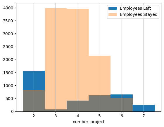
1 2 3 4 5 6 7 bins = np.linspace(1.5 , 7.5 , 7 ) plt.hist(df[df['left' ]==1 ]['number_project' ], bins=bins, alpha=1 , label='Employees Left' ) plt.hist(df[df['left' ]==0 ]['number_project' ], bins=bins, alpha=0.4 , label='Employees Stayed' ) plt.xlabel('number_project' ) plt.grid(axis='x' ) plt.legend(loc='best' );
项目少时离职了,可能因为员工锻炼机会少。
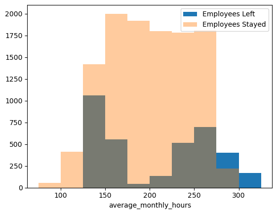
1 2 3 4 5 6 bins = np.linspace(75 , 325 , 11 ) plt.hist(df[df['left' ]==1 ]['average_monthly_hours' ], bins=bins, alpha=1 , label='Employees Left' ) plt.hist(df[df['left' ]==0 ]['average_monthly_hours' ], bins=bins, alpha=0.4 , label='Employees Stayed' ) plt.xlabel('average_monthly_hours' ) plt.legend(loc='best' );
工作时长少和多都容易离职。
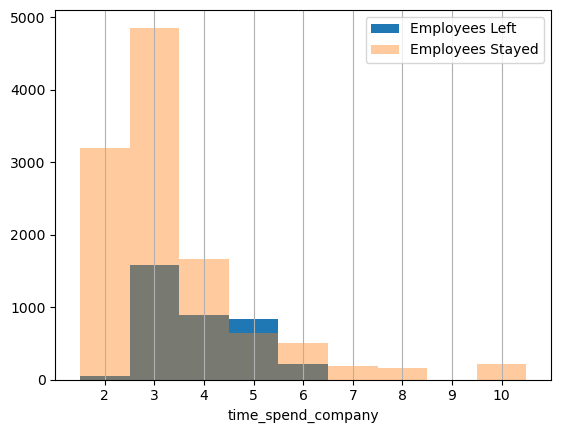
1 2 3 4 5 6 7 8 9 bins = np.linspace(1.5 , 10.5 , 10 ) plt.hist(df[df['left' ]==1 ]['time_spend_company' ], bins=bins, alpha=1 , label='Employees Left' ) plt.hist(df[df['left' ]==0 ]['time_spend_company' ], bins=bins, alpha=0.4 , label='Employees Stayed' ) plt.xlabel('time_spend_company' ) plt.xlim((1 ,11 )) plt.grid(axis='x' ) plt.xticks(np.arange(2 ,11 )) plt.legend(loc='best' );
工作年限3年,离职率最高。年限越长,离职率越低。
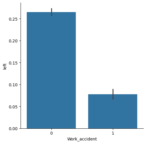
1 2 plot = sns.catplot(x='Work_accident' , y='left' , kind='bar' , data=df);
未发生工作事故的离职率较高,难以解释。
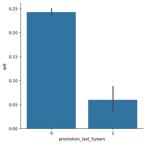
1 2 plot = sns.catplot(x='promotion_last_5years' , y='left' , kind='bar' , data=df);
不升职的离职率较高。
数据预处理 独热编码替换分类数据 1 2 3 4 5 6 7 8 9 10 11 12 13 14 15 X = df.drop('left' , axis=1 ) y = df['left' ] X.drop(['department' ,'salary' ], axis=1 , inplace=True ) salary_dummy = pd.get_dummies(df['salary' ]) department_dummy = pd.get_dummies(df['department' ]) X = pd.concat([X, salary_dummy], axis=1 ) X = pd.concat([X, department_dummy], axis=1 ) X.head()
satisfaction_level
last_evaluation
number_project
average_monthly_hours
time_spend_company
Work_accident
promotion_last_5years
high
low
medium
IT
RandD
accounting
hr
management
marketing
product_mng
sales
support
technical
0
0.38
0.53
2
157
3
0
0
False
True
False
False
False
False
False
False
False
False
True
False
False
1
0.80
0.86
5
262
6
0
0
False
False
True
False
False
False
False
False
False
False
True
False
False
2
0.11
0.88
7
272
4
0
0
False
False
True
False
False
False
False
False
False
False
True
False
False
3
0.72
0.87
5
223
5
0
0
False
True
False
False
False
False
False
False
False
False
True
False
False
4
0.37
0.52
2
159
3
0
0
False
True
False
False
False
False
False
False
False
False
True
False
False
拆分训练集和测试集 1 2 3 4 from sklearn.model_selection import train_test_splitX_train, X_test, y_train, y_test = train_test_split(X, y, test_size=0.3 )
数据标准化
比较大的数值,算法会认为其比较重要,导致结果不准确。
数值差异比较大的话,模型收敛较慢。
因此,需要将数据标准化。
1 2 3 4 5 6 7 8 9 10 from sklearn.preprocessing import StandardScalerstdsc = StandardScaler() X_example = np.array([[ 10. , -2. , 23. ], [ 5. , 32. , 211. ], [ 10. , 1. , -130. ]]) X_example = stdsc.fit_transform(X_example) X_example = pd.DataFrame(X_example) print (X_example)X_example.describe()
0 1 2
0 0.707107 -0.802454 -0.083658
1 -1.414214 1.409716 1.264429
2 0.707107 -0.607262 -1.180771
0
1
2
count
3.000000e+00
3.000000e+00
3.000000e+00
mean
-2.960595e-16
-1.110223e-16
7.401487e-17
std
1.224745e+00
1.224745e+00
1.224745e+00
min
-1.414214e+00
-8.024539e-01
-1.180771e+00
25%
-3.535534e-01
-7.048582e-01
-6.322145e-01
50%
7.071068e-01
-6.072624e-01
-8.365788e-02
75%
7.071068e-01
4.012270e-01
5.903856e-01
max
7.071068e-01
1.409716e+00
1.264429e+00
1 2 3 4 5 6 7 8 9 from sklearn.preprocessing import StandardScalerstdsc = StandardScaler() X_train_std = stdsc.fit_transform(X_train) print (X_train_std[0 ])X_test_std = stdsc.transform(X_test)
[ 1.40697692 -0.21068428 -0.65422416 -1.37529896 -1.02172591 -0.41080801
-0.14595719 -0.30564365 -0.98084819 1.16499228 -0.2981308 -0.23781569
-0.22665375 -0.23057496 -0.21332806 -0.24641294 -0.25073288 1.62416352
-0.41712208 -0.47247431]
构建模型 随机森林法 1 2 3 4 5 6 7 8 9 10 11 12 13 14 15 16 17 18 19 20 21 22 from sklearn.model_selection import ShuffleSplitcv = ShuffleSplit(n_splits=20 , test_size=0.3 ) from sklearn.ensemble import RandomForestClassifierfrom sklearn.model_selection import GridSearchCVrf_model = RandomForestClassifier() rf_param = {'n_estimators' : range (1 ,11 )} rf_grid = GridSearchCV(rf_model, rf_param, cv=cv) rf_grid.fit(X_train, y_train) print ('Parameter with best score:' )print (rf_grid.best_params_)print ('Cross validation score:' , rf_grid.best_score_)
Parameter with best score:
{'n_estimators': 9}
Cross validation score: 0.9835079365079364
1 2 3 best_rf = rf_grid.best_estimator_ print ('Test score:' , best_rf.score(X_test, y_test))
Test score: 0.9884444444444445
1 2 3 4 5 6 7 8 features = X.columns feature_importances = best_rf.feature_importances_ features_df = pd.DataFrame({'Features' : features, 'Importance Score' : feature_importances}) features_df.sort_values('Importance Score' , inplace=True , ascending=False ) features_df
Features
Importance Score
0
satisfaction_level
0.260366
3
average_monthly_hours
0.186585
2
number_project
0.179788
4
time_spend_company
0.179571
1
last_evaluation
0.144083
5
Work_accident
0.011949
8
low
0.006395
7
high
0.005206
9
medium
0.003336
17
sales
0.003200
18
support
0.003070
19
technical
0.003039
11
RandD
0.002143
10
IT
0.002048
12
accounting
0.001887
6
promotion_last_5years
0.001799
14
management
0.001755
13
hr
0.001425
16
product_mng
0.001182
15
marketing
0.001173
1 2 features_df['Importance Score' ][:5 ].sum ()
np.float64(0.9503925098929926)
基于聚类模型的分析 1 2 3 4 5 6 7 import numpy as npimport pandas as pdimport matplotlib.pyplot as pltimport seaborn as sns%matplotlib inline data = pd.read_csv(url)
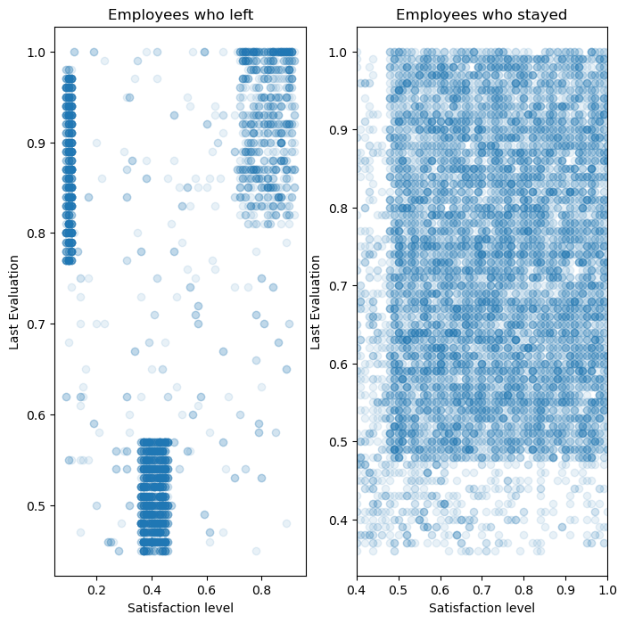
1 2 3 4 5 6 7 8 9 10 11 12 13 plt.figure(figsize = (8 ,8 )) plt.subplot(1 ,2 ,1 ) plt.plot(data.satisfaction_level[data.left == 1 ],data.last_evaluation[data.left == 1 ],'o' , alpha = 0.1 ) plt.ylabel('Last Evaluation' ) plt.title('Employees who left' ) plt.xlabel('Satisfaction level' ) plt.subplot(1 ,2 ,2 ) plt.title('Employees who stayed' ) plt.plot(data.satisfaction_level[data.left == 0 ],data.last_evaluation[data.left == 0 ],'o' , alpha = 0.1 ) plt.xlim([0.4 ,1 ]) plt.ylabel('Last Evaluation' ) plt.xlabel('Satisfaction level' )
Text(0.5, 0, 'Satisfaction level')
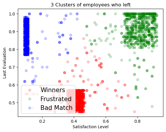
1 2 3 4 5 6 7 8 9 10 11 12 13 14 15 16 from sklearn.cluster import KMeanskmeans_df = data[data.left == 1 ].drop([ u'number_project' , u'average_montly_hours' , u'time_spend_company' , u'Work_accident' , u'left' , u'promotion_last_5years' , u'sales' , u'salary' ],axis = 1 ) kmeans = KMeans(n_clusters = 3 , random_state = 0 ).fit(kmeans_df) kmeans.cluster_centers_
array([[0.41014545, 0.51698182],
[0.80851586, 0.91170931],
[0.11115466, 0.86930085]])
1 2 3 4 5 6 7 8 9 10 11 12 13 14 15 16 17 18 19 20 21 22 23 24 25 26 27 28 29 left = data[data.left == 1 ] left_labels = (data.left == 1 ) data.loc[left_labels, 'label' ] = kmeans.labels_ left = data[data.left == 1 ] plt.figure() plt.xlabel('Satisfaction Level' ) plt.ylabel('Last Evaluation' ) plt.title('3 Clusters of employees who left' ) plt.plot(left.satisfaction_level[left.label==0 ], left.last_evaluation[left.label==0 ], 'o' , alpha=0.2 , color='r' ) plt.plot(left.satisfaction_level[left.label==1 ], left.last_evaluation[left.label==1 ], 'o' , alpha=0.2 , color='g' ) plt.plot(left.satisfaction_level[left.label==2 ], left.last_evaluation[left.label==2 ], 'o' , alpha=0.2 , color='b' ) plt.legend(['Winners' , 'Frustrated' , 'Bad Match' ], loc=3 , fontsize=15 , frameon=True );
加关注 关注公众号“生信之巅”
敬告 :使用文中脚本请引用本文网址,请尊重本人的劳动成果,谢谢!Notice : When you use the scripts in this article, please cite the link of this webpage. Thank you!